Building a Racing-Line Playground
I enjoy racing, and I program professionally. The Line is where those interests meet: a little physics playground for asking why one line through a corner works better than another. It has the same appeal as fluid. Drag something, change a parameter, and watch the consequences. A line on a road becomes much more interesting when there is a speed trace beneath it and a ghost showing what changed.
The result is a Go application with a native Ebitengine viewer, twelve fictional tracks, editable car setups, authored lines, pinned references, and a CLI that exports images, animations, and numerical results. The fun is in making a small change and following its consequences through the corner.
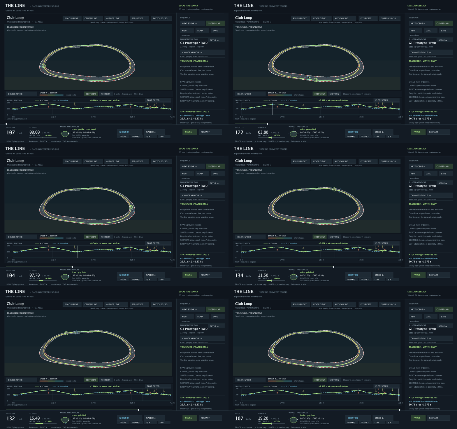
A road needs more than a smooth outline
The road begins as control points carrying position, width, banking, surface, and kerb information. A natural cubic spline joins an open sequence; a periodic cubic closes a circuit. Both keep position and the first two derivatives continuous at the joins. That matters because curvature drives the car’s lateral demand. A small geometric kink can become a large, artificial speed restriction.
Width and bank interpolate smoothly without overshooting their endpoint values. Surface changes remain categorical. The sampled road becomes a triangle ribbon, and a candidate trajectory follows that surface, including triangle crossings and actual three-dimensional segment lengths.
Clearance needed more care than simply subtracting half a car width from each cross-section. A line can fit those cross-sections and still clip a tapering edge between them. The implementation checks the swept circular footprint against actual side-edge segments, including nearby cells. Kerb contact uses the same indexed geometry to determine grip.
Changing the centreline interpolant taught me another useful distinction: smooth curvature does not imply one tidy speed minimum per corner. The searched esses line still has small secondary extrema. Those remain visible in the chart, where they can tell us something about the path and the search.
Turning and braking share the same grip
For a flat, steady corner, the useful starting point is lateral acceleration:
a_lateral = speed² × curvature
Doubling speed asks for four times the lateral acceleration on the same curve. Making the path wider can reduce curvature, but also adds distance. The fastest path has to balance those effects over the whole sequence.
Tyres also need longitudinal force to accelerate or brake. A simple friction circle expresses the shared budget:
longitudinal_force² + lateral_force² <= (grip × normal_load)²
The model applies axle limits alongside engine power, a braking cap, drag, and signed gravity contributions from grade and bank. A fixed front/rear drive split means unused grip on one axle cannot automatically help the driven axle. Banking can help a turn in one direction and hurt it in the other.
The model is quasi-static: it asks which forces are feasible at a position and speed. Its road, GT, and rally cars are illustrative setups. Steering transients, tyre slip curves, suspension motion, and tyre temperature would require additional state and a different level of modelling. Within this scope, changing grip, weight, power, or drive split has a concrete effect that the viewer can expose.
The next corner tells you when to brake
Once a path is chosen, the solver finds lateral speed ceilings and propagates acceleration and braking constraints along it. A forward pass limits what the car can reach; a backward pass limits what it can slow down from before the next restriction. Braking for a tight corner therefore starts upstream, and a low-grip patch can influence the approach before the car reaches it.
The segment calculation uses squared-speed kinematics:
next_speed² = speed² + 2 × acceleration × segment_length
Force bounds change with speed and position, so segment interiors need checking too. Nonconstant segments begin with five envelope samples and are checked at 65 points before acceptance. A failed check raises that segment’s working resolution and recomputes the profile.
Around that evaluator sits a deterministic search over smooth lateral-offset bumps. It tries changes at decreasing amplitudes, keeps feasible improvements, and reevaluates a shortlist on a road sampled at 0.5 m or finer. The verified centreline remains a fallback. This produces a useful heuristic estimate of a fast line; the search budget and grid can affect which local solution it finds.
One recorded default-budget esses run reduced the centreline’s 15.8486 seconds to 14.2406 seconds, a 10.15% improvement under the same car and boundary caps. Reevaluating that chosen path at 0.25 m changed its time by 0.010%. Those are two separate observations: searching found a faster path, and refining that path barely changed its evaluated time. The validation record keeps both measurements explicit.
A little axle modelling goes a long way
The optional setup page adds fixed brake bias, downforce and its front/rear balance, longitudinal load transfer, and tyre load sensitivity. These make some familiar handling questions possible without introducing a full suspension simulation.
With positive drive force, longitudinal transfer reduces front normal load and increases rear normal load. Braking reverses that shift. The amount depends on tyre force times CG height divided by wheelbase. That makes front-wheel-drive and rear-wheel-drive launch limits behave differently, and gives brake bias something meaningful to interact with.
Downforce grows with speed squared and is divided between the axles by aero balance. Lateral force allocation still follows the steady yaw-moment balance implied by the static CG position. Adding all the downforce to the rear can leave the front axle as the cornering bottleneck. The richer model’s utilization display therefore reports the most heavily used axle; spare rear capacity cannot conceal an overloaded front.
Load sensitivity makes capacity grow less than proportionally with normal load. That turns some explicit force bounds into a small numerical root problem. The implementation uses a bracketed Newton solve with bisection fallback and returns a checked feasible bound. An independent grid reconstructed 8,000 signed axle limits and measured a maximum active-constraint residual of 2.66 × 10⁻¹¹ m/s², with forces expressed per unit vehicle mass. That checks the numerical solution of the declared model. Real-car calibration is a separate question.
One particularly useful experiment is to vary downforce and drag independently. The model has separate parameters for them, so adding downforce alone leaves a power-limited straight-line top speed unchanged when drag is held fixed. To explore an aero tradeoff, change both. The vehicle model notes spell out the equations and conventions.
A lap has no convenient starting speed
An open road has entry and exit speed caps. A circuit needs the end of the lap to join the beginning with the same state. Club Loop therefore uses a periodic road and cyclic speed propagation: each forward/backward pass carries reductions across the seam until speed changes fall below 0.000001 m/s. The solve has a 40-pass bound and reports failure if it does not converge.
Playback has a related wrinkle. Each car wraps by its own lap duration. The faster line can begin its next lap while the reference is still finishing the previous one. The chart continues to compare one-lap elapsed times at matching road stations, which is a different quantity from the cars’ accumulating race gap.
Profiling the repeated question
The expensive question is “how fast can this car follow this path?” Search asks it repeatedly. Profiling the default road-car esses solve put 68.5% of sampled CPU time in segment-envelope work, including repeated trigonometry and copies of the force-instrumentation payload.
Caching immutable road-frame projections, using compact bounds during profile work, reusing segment storage, and avoiding redundant envelope calculations reduced that workload substantially. Independent finalists can also run in a bounded native worker pool. Results are consumed in a fixed order so scheduling does not choose the winning line; the dependent coordinate-search steps remain sequential. Browser/WASM evaluation uses one worker and cooperatively yields to the event loop.
The recorded September 10 measurements used Go 1.24.0 on macOS/amd64, Intel Core i5-1038NG7. Each was a single benchmark iteration; the final measurements ran without competing test or solve processes:
| Workload | Elapsed time | Allocated memory |
|---|---|---|
| Default road-car esses search, before profiling changes | 4.246 s | 67.90 MB |
| Default road-car esses search, after changes | 1.564 s | 111.22 MB |
| Centreline evaluation, cold cache, after changes | 41.42 ms | 9.17 MB |
| Richer axle-model esses search, after changes | 45.269 s | 103.05 MB |
The default solve was 2.71 times faster in that comparison, with more total allocation because of the cached projections. The richer case enabled fixed brake bias, load transfer, load sensitivity, and downforce; its exact setup and benchmark commands are in the performance record. These measure solve latency, not animation frame rate.
The remaining cost shaped the interface. Even cold centreline evaluation missed the 16 ms provisional-result target, so evaluation and search run asynchronously and support cancellation. A setup edit first evaluates the existing line, then searches for an improvement. If a wider car makes that old line invalid, the editor retries with a fresh search. Later edits supersede earlier work, and stale replies cannot overwrite the current scene.
I also kept verification independent of the performance shortcuts. Tests reconstruct forces from exported geometry and kinematics, while deterministic fixture comparisons check that the faster default path preserves the recorded trajectories. The search notes describe the evaluation density, worker boundaries, and reproducible profiling commands.
Make the comparison part of the toy
A pinned reference is what turns a moving car into an experiment. Pin the current run, change one setting, and scrub the chart at the same road station. A negative elapsed-time delta means the new line got there sooner. The ghost answers the complementary question: where was the other car at this same elapsed time?
You can also drag an authored line and test an idea directly. Opening the exit, sacrificing the first part of an esses, or changing the bank becomes a hypothesis with a visible consequence. Saving the study preserves the setup and reference so the comparison can be revisited.
That is the part I enjoy most about these little physics projects. The equations become controls, and the controls make the equations easier to question. The repository’s quick start gets the viewer running; the default esses is a good place to pin a ghost, move a corner, and see what happens.